Raw sensor data and the labels that come with real fieldwork rarely line up cleanly. We had to build the full path from collection through modeling and into outputs that could be reviewed and challenged.
Sensors capture detailed curves across many narrow bands. Minerals leave distinct signatures in those curves that standard imaging misses. Conditions in the field shift constantly, and labels often come from different methods that don't always agree. Small classes matter most, yet they are easy to miss in the overall picture.
The sensor gives you spectra
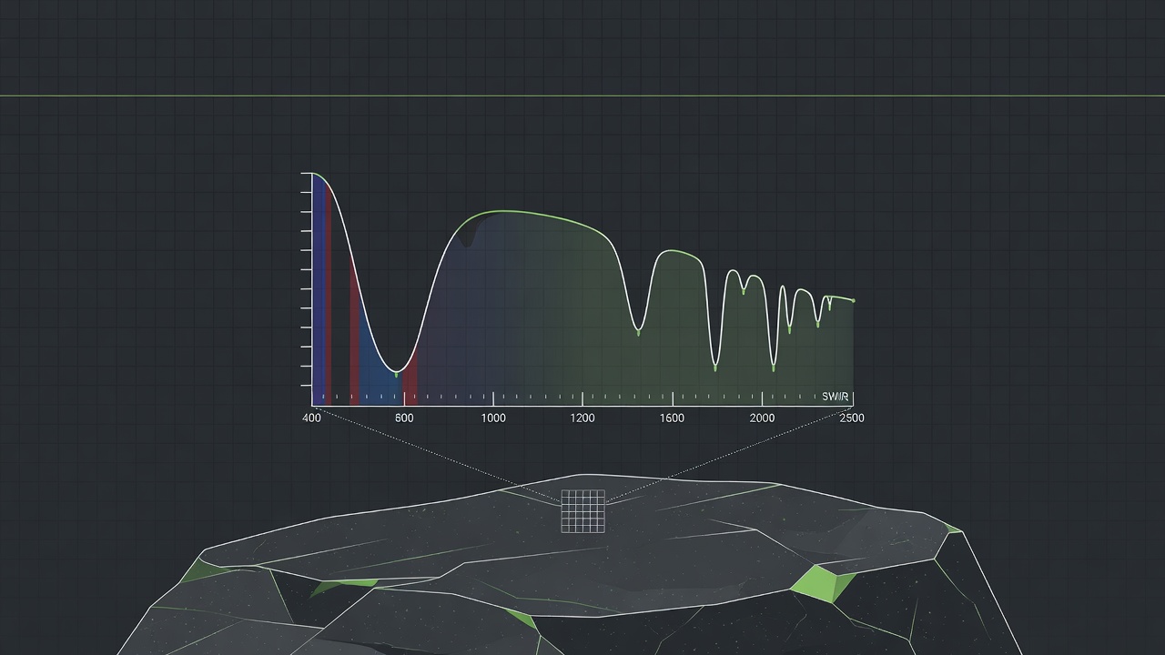
Hyperspectral sensors just dump reflectance numbers across hundreds of narrow bands. Visible through shortwave infrared. One pixel is basically a full curve. Different minerals create absorption dips that RGB cameras completely miss. The physics is not the mystery. Getting from the raw dump to something you can trust is where everything breaks or works.
On site the conditions never stay still. Labels came from physical samples or direct observation. Annotators disagreed on the same pixel all the time. Mask conventions drifted between people. The actual target pixels were often a tiny fraction of the whole scene. You could hit high overall accuracy and still be completely wrong on the classes that mattered.
The labels fought back
Careful checking of every training mask against the actual values caught mismatches that would have silently corrupted training. Class imbalance was extreme, so sampling and augmentation came first — rotations, noise, stretching the curves — before architecture choices could be compared fairly.
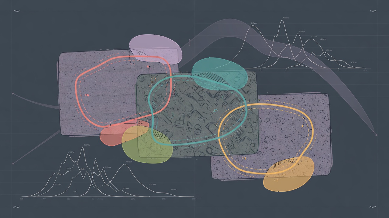
Per-class precision, recall, and F1 made the problem obvious fast. The sparse classes were getting crushed. Other measures cut through the imbalance that plain accuracy hides.
Adding space to the spectrum
Looking at one pixel in isolation throws away the geology. A zone next to a different feature carries different meaning than the same signature sitting alone. We ran one stream on the reflectance curve itself and another on the local patch. Patch size became something we tuned to the actual scale of the features we cared about.
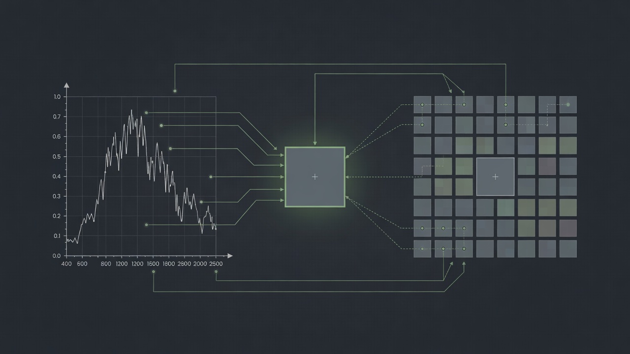
A reference comparison gave a sanity check we could discuss in the same terms as the sensor. When the model and the reference disagreed on a pixel that looked right spatially, that told us where to dig.
The maps hide the hard parts until you look close
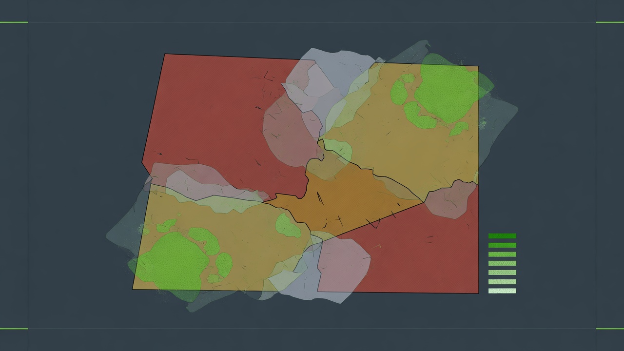
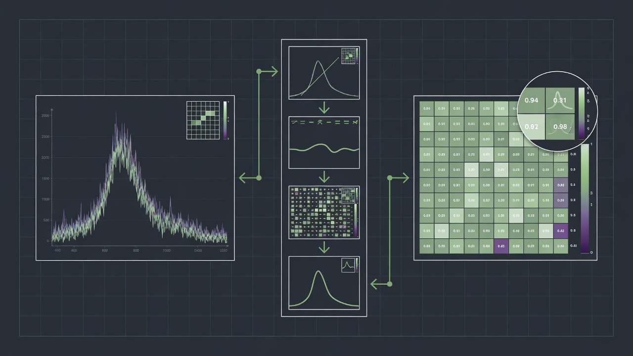
The pictures told us more than the numbers. Overlays and confidence maps made the fuzzy boundaries visible. Most of the bad errors happened at contact zones where the sensor was seeing mixed materials and the labels were already fuzzy. Confusion patterns showed which classes overlapped most.
Letting people see the wobble
If someone is actually going to use this, they need to see the raw data and the doubt. Raw curves, the steps we took, per-pixel confidence. If you hide the uncertainty, people eventually stop trusting the output.
The label work and those boundary cases are what decide whether any of this ever gets used. Once we had some handle on those, the modeling part felt almost secondary.
We are still early on this kind of work. The interesting problems are rarely the ones that look clean in a slide.